GIS Crime Hotspot Analysis: A Step-by-Step ArcGIS Pro Tutorial

Build a crime-analysis project from a fixed Chicago dataset: import incidents, check the locations, count incidents by community area, calculate Getis-Ord Gi* hot spots, optionally create a density raster, and export a map. All settings and checkpoints are included below; no separate help article is needed to follow the workflow.

Software: ArcGIS Pro with a valid licence. Spatial Analyst is required only for the optional Kernel Density step. Study: reported BURGLARY incidents in Chicago during calendar year 2024. Analysis: incident counts, not population-adjusted crime risk.

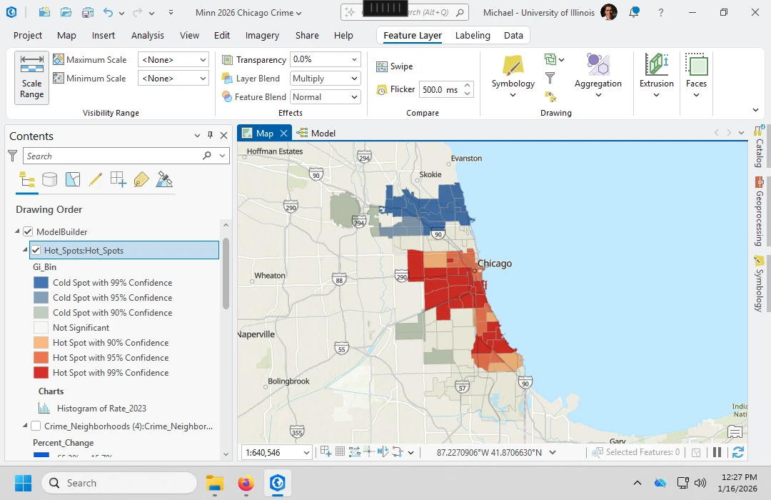
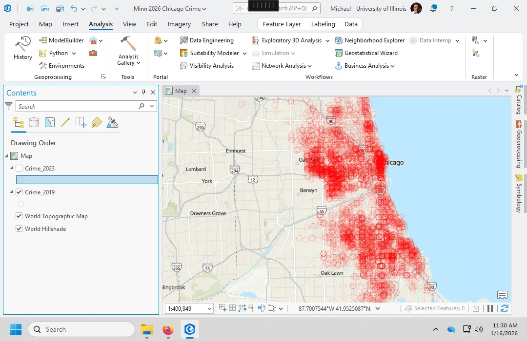
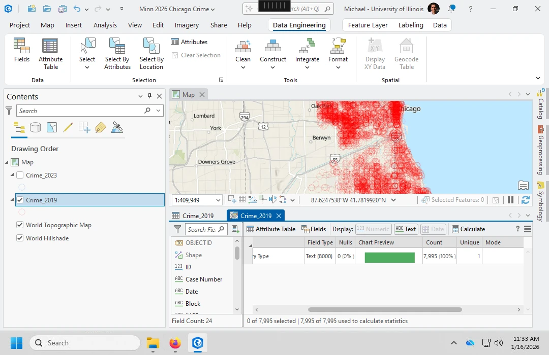
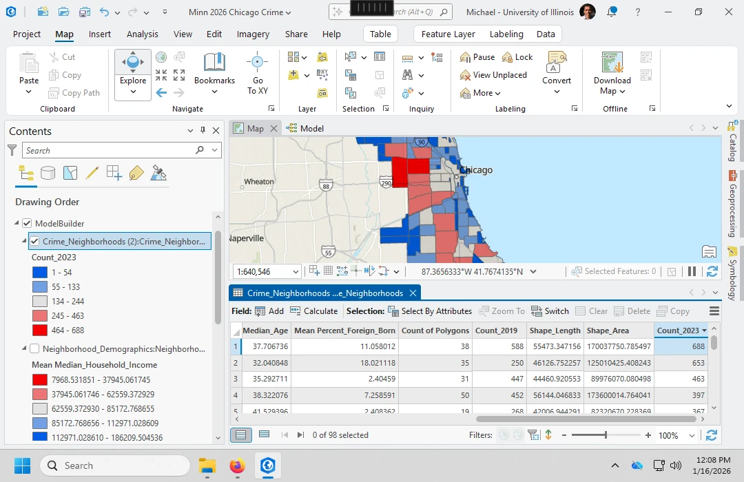
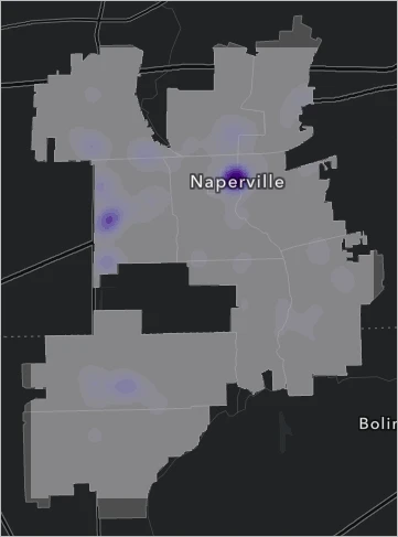
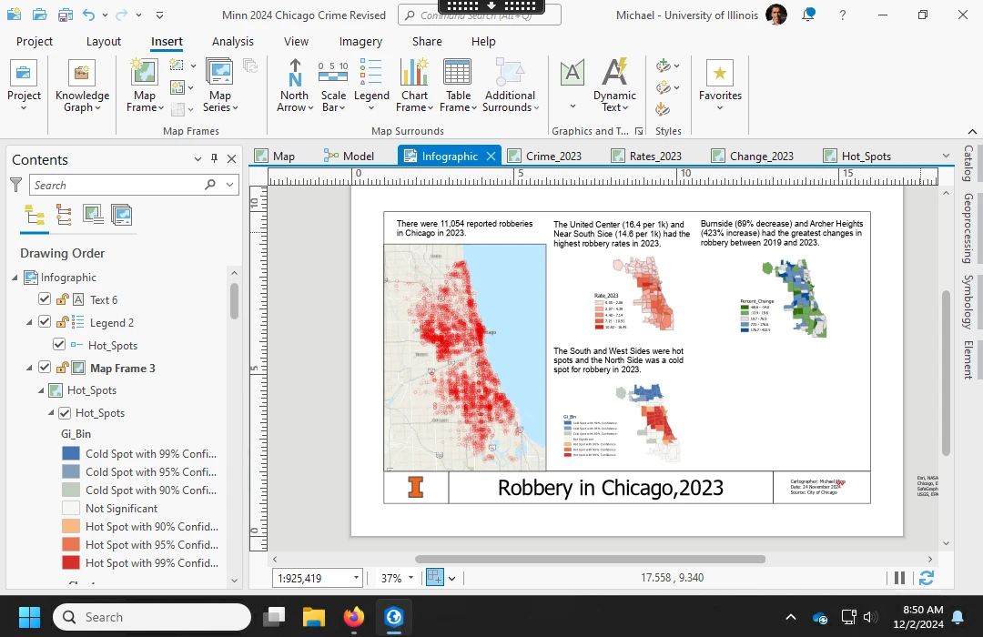
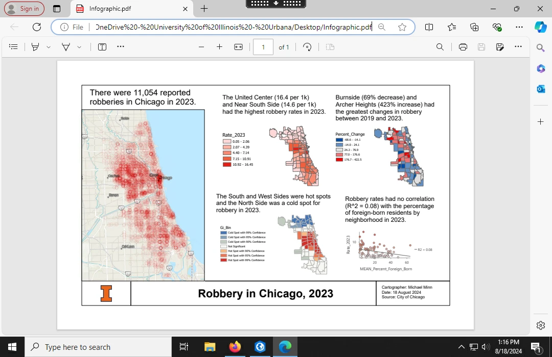
About the screenshots: these are real screenshots from published ArcGIS articles, credited beside each image. They illustrate the tools and output types. Michael Minn's screenshots use Chicago robbery data from other years; Esri's density example uses fictitious Naperville data. They are not screenshots of the supplied burglary dataset. Follow the written settings below rather than copying example layer names, values, or map patterns from the images.

1. Download the complete practice package

Download the Spatialtuts crime-hotspot dataset and analysis script (ZIP). Extract it to a writable folder, for example C:\GIS\Spatialtuts. Do not run tools against files still inside the ZIP.

The package contains:

• burglary_2024.csv: 8,396 unique records with usable longitude and latitude.
• areas.geojson: 77 Chicago community-area polygons in WGS 84.
• run_analysis.py: the complete ArcPy workflow, including reconciliation checks.
• data-checks.json and sources.json: extraction totals, source queries, and retrieval date.
• README.txt: local execution instructions.

The source query returned 8,436 records; 40 had missing or invalid coordinates and were excluded from the CSV. Distinct incidents sharing a location were retained. The data comes from the City of Chicago's Crimes dataset and its community-area boundary dataset. The packaged snapshot avoids later portal updates changing your input counts.

2. Create a project and import the points

1. In ArcGIS Pro, create a new Map project named Chicago_Burglary_2024.
2. Open Analysis > Tools and search for XY Table To Point.
3. Set Input Table to burglary_2024.csv, X Field to longitude, and Y Field to latitude.
4. Set Coordinate System to GCS WGS 1984 (EPSG:4326). Leave Z Field empty.
5. Save the output in the project geodatabase as incidents_wgs84, then click Run.
6. Run JSON To Features with areas.geojson, Geometry Type Polygon, and output areas_wgs84.

Checkpoint: the point table should contain 8,396 records and the polygon table 77. If the points appear on another continent, check that X is longitude, Y is latitude, and the input system is WGS 84. A city basemap is optional and is not used in any calculation.

3. Project both layers into metres

Run Project twice. Use output coordinate system WGS 1984 UTM Zone 16N (EPSG:32616). Project incidents_wgs84 to incidents_utm, and areas_wgs84 to areas_utm. Both use the WGS 84 datum, so this workflow does not need a datum change.

Use Project, not Define Projection: the former transforms coordinates; the latter only changes their coordinate-system description. In each output's Layer Properties > Source, verify EPSG:32616 and metre units. Keep the two original WGS 84 layers for comparison, but use the projected copies for the remaining analysis.

4. Audit boundary matches before counting incidents

This step prevents double-counting incidents on shared boundaries and avoids treating locations outside the study area as valid community-area observations.

1. Run Spatial Join with Target Features incidents_utm and Join Features areas_utm.
2. Choose Join one to one, keep all target features, and Match Option Intersect. Name the output point_boundary_audit.
3. Open the output table and examine Join_Count. Zero means no community polygon matched; a value above one means an ambiguous match.
4. Select records where Join_Count = 1 and export the selection as analysis_points.
5. Record the numbers excluded for zero and multiple matches. These spatial exclusions are separate from the 40 coordinate exclusions made before the download.

Checkpoint: every retained analysis point now has exactly one matching community area. Its feature count may be lower than 8,396. Keep the audit layer so the exclusions remain reviewable.

5. Count incidents in all 77 community areas

Run another Spatial Join, this time with Target Features areas_utm and Join Features analysis_points. Set Join one to one, keep all target features, and Match Option Intersect. Save the output as community_counts.

Keep Join_Count, the incident count, and the community name field. Symbolize the polygons using Graduated Colors on Join_Count to see the count distribution. Preserve zero-count polygons; they are valid observations.

Checkpoint: there must still be 77 rows. Summing Join_Count across the polygons must equal the feature count of analysis_points. If those totals differ, stop and inspect the boundary audit before running statistics.

6. Calculate statistically significant hot and cold spots

Open Hot Spot Analysis (Getis-Ord Gi*) and enter the following specification:

Parameter	Value for this tutorial
Input Feature Class	community_counts
Input Field	Join_Count
Output Feature Class	community_hotspots
Conceptualization of Spatial Relationships	K nearest neighbors
Number of Neighbors	8
Distance Method	Euclidean
Apply False Discovery Rate Correction	Checked

The eight-neighbor specification is an explicit teaching choice, not a claim that eight is optimal for Chicago. It avoids copying an undocumented automatically chosen distance. Run the tool, retain its messages, and inspect the 77 output polygons.

Use Gi_Bin for the FDR-corrected significance map. Positive classes are hot spots, negative classes are cold spots, and zero is not statistically significant. Absolute values 1, 2, and 3 represent the tool's 90%, 95%, and 99% categories. GiZScore and GiPValue contain unadjusted statistics; do not substitute their raw thresholds for the corrected classification.

Checkpoint: the output contains 77 polygons and the three fields named above. No particular number of red polygons is promised. A legitimate run may find few significant areas. A cold spot does not mean zero crime, and a neutral polygon does not prove safety.

7. Create the optional density raster

This step needs the Spatial Analyst extension. If it is unavailable, your Getis-Ord analysis remains complete; continue to the layout step without a density raster.

1. Run Dissolve on areas_utm with no dissolve field. Save study_boundary.
2. Open Kernel Density. Set input to analysis_points, Population Field to None, Output Cell Size to 100, Search Radius to 2000, Area Units to Square kilometers, Output Cell Values to Densities, and Method to Planar.
3. On Environments, use EPSG:32616, Extent study_boundary, and Mask study_boundary.
4. Save as burglary_density.tif. Display it with a light-to-dark sequential color scheme and a readable legend.

These values mean 100-metre pixels and a 2,000-metre smoothing radius. They are fixed exercise settings, not an optimized risk model. The raster estimates incident density per square kilometre, not population-normalized risk. It answers a different question from the Gi* significance map.

8. Assemble and export the final map

1. Choose Insert > New Layout and select A4 landscape.
2. Insert a map frame showing community_hotspots. Add a second frame for community_counts, and a third for the density raster if available. Use separate maps or fixed layer visibility for the frames so changing one does not unexpectedly change the others.
3. Add a title: Recorded Burglary in Chicago, 2024. Include legends identifying incident counts, FDR-corrected Gi* classes, and density units.
4. Add a scale bar, north arrow, data source, and the snapshot date from sources.json.
5. Add a note: Reported incidents; generalized locations; counts are not population-adjusted risk. Eight nearest neighbors; FDR enabled.
6. Save the project, then choose Share > Export Layout. Export a PDF and a PNG at 300 dpi.

Run the entire analysis with the included script

For a reproducible tool sequence, open View > Python Window inside ArcGIS Pro and paste the following two lines. Change only the path to the extracted folder:

import runpy
runpy.run_path(r"C:\GIS\Spatialtuts\run_analysis.py", run_name="__main__")

The script creates a new timestamped output folder instead of overwriting previous work. It imports and projects the data, audits boundary matches, retains unambiguous points, counts incidents, verifies reconciliation, calculates the eight-neighbor/FDR hot spots, and exports hotspot_results.csv. When Spatial Analyst is available, it also writes burglary_density.tif. It logs skipped density generation explicitly when the extension is unavailable.

The script has been syntax-checked but has not been executed in licensed ArcGIS Pro here. The sourced screenshots are reference examples, not proof of a completed run of this snapshot.

What you should have at the end

• A saved ArcGIS Pro project with the source and projected data.
• The point_boundary_audit layer and documented exclusions.
• analysis_points and 77 community_counts polygons with reconciled totals.
• 77 community_hotspots polygons containing GiZScore, GiPValue, and Gi_Bin.
• An optional 100-metre density raster using a 2,000-metre radius.
• A labelled PDF/PNG map layout.
• For script runs, hotspot_results.csv and audit.json alongside the file geodatabase.

Troubleshooting: no points usually indicates wrong XY fields or a bad input path. Degree-sized coordinates in the projected outputs indicate the wrong tool or coordinate system. A failed count reconciliation requires checking the boundary audit. Missing density output requires checking the Spatial Analyst licence. Few or no significant hot spots can be a valid statistical result; do not change settings merely to force a red map.

Use the results to describe the recorded spatial pattern and its uncertainty. Reporting practices, missing records, aggregation, and neighborhood choices influence the map; none of these outputs establishes causation or predicts an individual's behavior.